Use formulas to fill out a budget
Introduction (00:04)
Excel is a fantastic tool for calculating numbers. You have a wide range of functions and formulas to choose from. In this video you’ll learn how to use basic calculations to fill out a marketing budget template. You’ll also learn some shortcuts for how to quickly fill your spreadsheet with numbers, how to calculate sums and how to use absolute and relative references. Let me show you:
Using “autofill” to automatically fill cells with values (00:31)
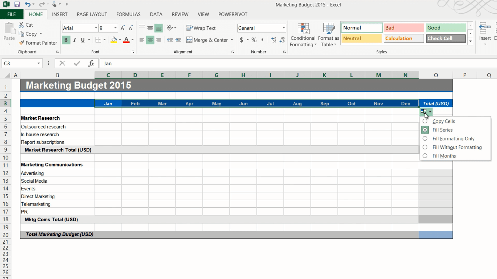
Here I have a simple template for a marketing budget for 2015 that I need to fill out. My template doesn’t have the months so I’ll add them to the third row. You can save time by letting Excel automatically fill the cells for you. To use autofill, start writing the first cell, here I’ll write “Jan”. To continue filling in the rest of the months, position your mouse pointer in the bottom right corner of the cell and drag the fill handle to the right. You can use autofill for time series like months, days and quarter, but you can also use it for numbers and other sequences. A little autofill icon appears where you can choose if you want to copy cells or fill the series. I am happy with this so I will just move on.
Now I’ll add the first budget item which is “Outsourced research”. We pay a fixed cost of 500 dollars a month for this so I’ll write 500 in the first cell and then copy the number across all months by dragging the fill handle. Again I can change the autofill options in the drop down if I wanted to.
Using a formula to apply a 20% increase (01:34)
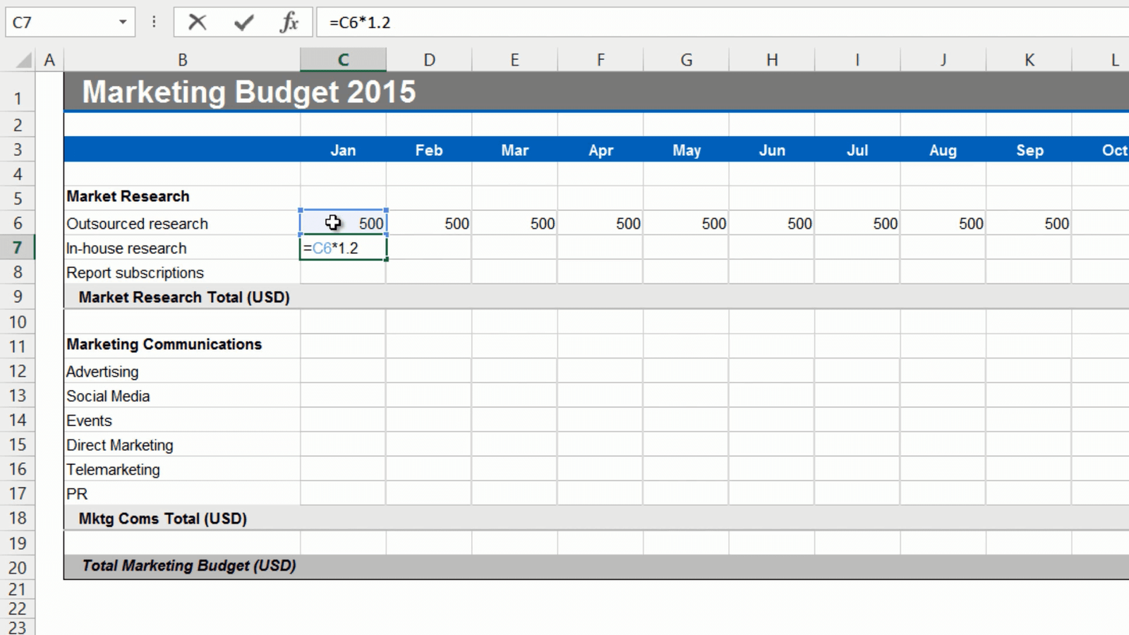
The next item, the “In-house research” is 20 percent more expensive than the outsourced market research so I’ll create a formula to calculate that number. To insert a formula, mark the cell and write an equal sign, this is the way you start all formulas in Excel, then I’ll mark the “Outsourced research” number and multiply it with 1.2 to get the 20 percent increase and press “Enter” to see the result.
There, that looks fine, so now I’ll grab the fill handle and drag it across all columns to copy the formula. If you double-click one of the cells you can see that the formula takes the value above and multiplies it with 1.2. This is a so called relative reference, meaning that the formula is updated to reflect its location in the spreadsheet.
Filling multiple cells at once with the same value (02:25)
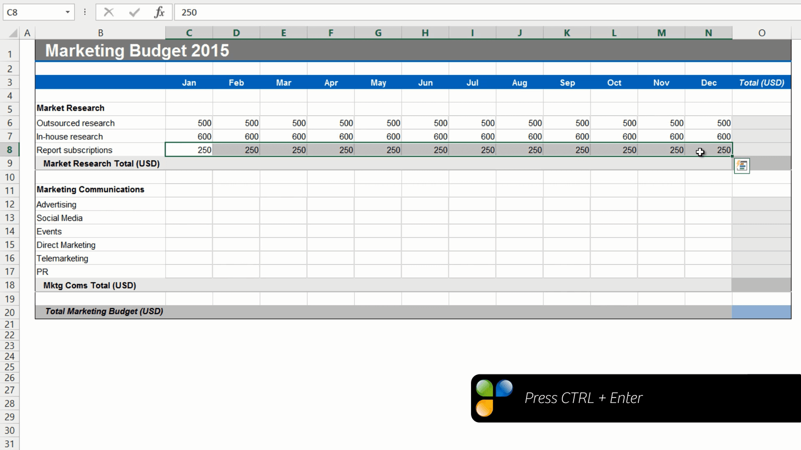
Next I want to fill out the “Report subscription” row. This is a fixed cost of 250 dollars each month. Instead of entering the number in the first cell and using autofill, you can mark all the cells where you want the value, write the number, here I will write 250 and press “CTRL + Enter”.
All the cells are filled at once.
Using “AutoSum” to calculate totals (02:46)
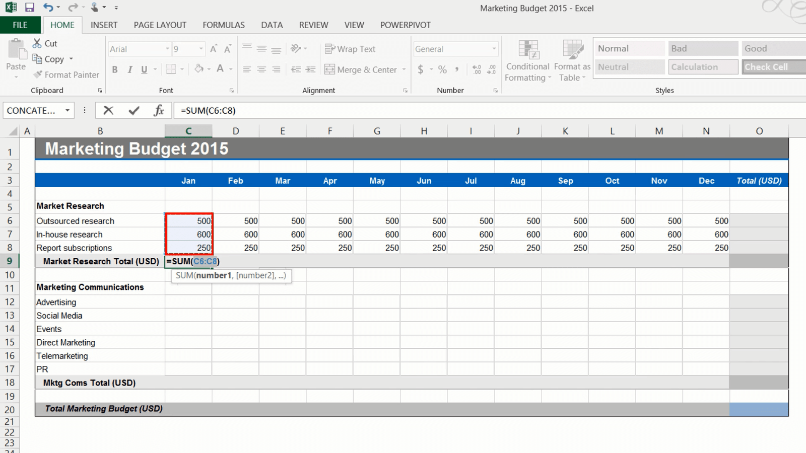
Now I want to add totals for this section. Since adding up numbers is done very frequently in Excel, there is a button for it called “Autosum”. To use Autosum, mark the cell where you want the total on the “HOME” tab, in the “Editing” section click the “AutoSum” icon with the Greek symbol Sigma (S).
Autosum will automatically select all numbers in the adjacent data range. In this case cells C6 to C8. Press “Enter” to see the result. To get the totals for the rest of the months, you can copy the Autosum formula by dragging the fill handle to the right. To use Autosum for the row totals, position the marker in the first row total and click “AutoSum”. As you can see the data range to the left is selected and summarized.
If you have numbers in a data range like this and you want to add totals for both rows and columns, you can save time by marking the entire data range, including the empty cells where you want to have the totals, and clicking “AutoSum”. All the totals you need are added in a split second.
Using formulas with fixed, “absolute” references (03:54)
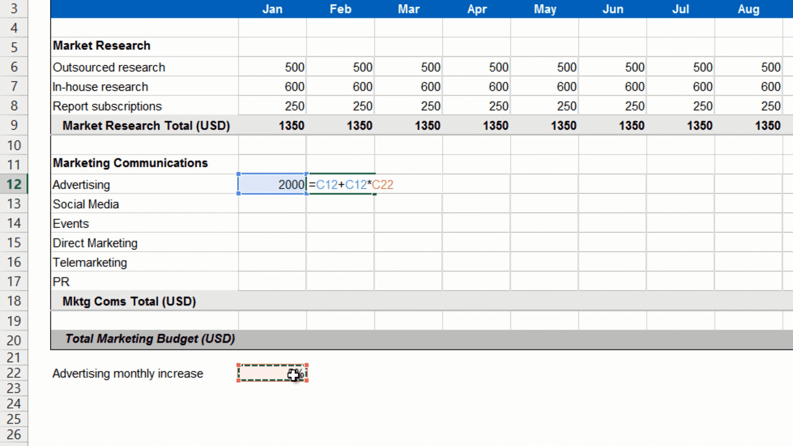
In the next section the first line item is “Advertising”. I want to incrementally increase the advertising with a certain percentage each month. I’ll start with 2000 dollars in January. I’ll mark the year total and click “Autosum”. Now I want to test some different percentage increases to see what the total cost will be for the year. Under my budget I’ll write, “Advertising monthly increase” and just start out with a percentage, let’s try 5%.
I’ll mark the cell next to the first month’s spend and write the formula, equal sign, previous month, plus previous month times the percentage increase and press enter to see the result.
If you want to copy this formula, that includes the reference to the percentage in cell C22 to other cells, you need to use an absolute reference. If you don’t, and try to copy this formula across the rows you won’t get the right results. If you double-click the formula you can see that the formula is using the value in the cells one step to the right, so it’s not picking up the 5 percent increase. To get the right result you need to change the formula so that it uses an absolute reference for the percentage increase. Double-click the cell with the formula, position your marker on the cell reference for the percentage increase, in this case it is Cell C22. To make this an absolute reference add a dollar sign before the column letter and row number to keep it fixed. The easiest way to do that is to press “F4” on your keyboard and then press “Enter”. Now you can apply the formula to the entire row and you will get the correct result.
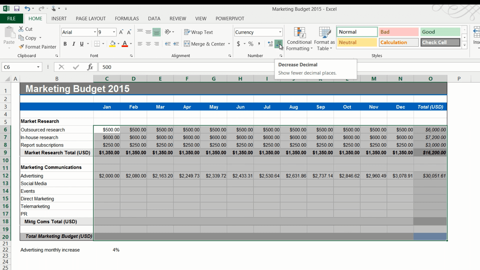
As you can see the total is much more than 30,000 which is more than I want to spend but now I can easily just change the percentage to say 4 percent. The total is now slightly higher than 30,000, but that’s ok, I’ll leave it like that.
Changing the number format (05:49)
Now I got a lot of decimals that I don’t need. First I’ll change the number format to currency, to do that, mark the cells where you have the numbers, on the “HOME” tab in the “Number” section I’ll select “Currency”. I’ll leave the default which is US dollars. Then I’ll reduce the number of decimals by clicking “Decrease Decimal” in the “Number” section. This doesn’t delete the decimals it just hides them.
Removing formulas and keeping the values (06:14)
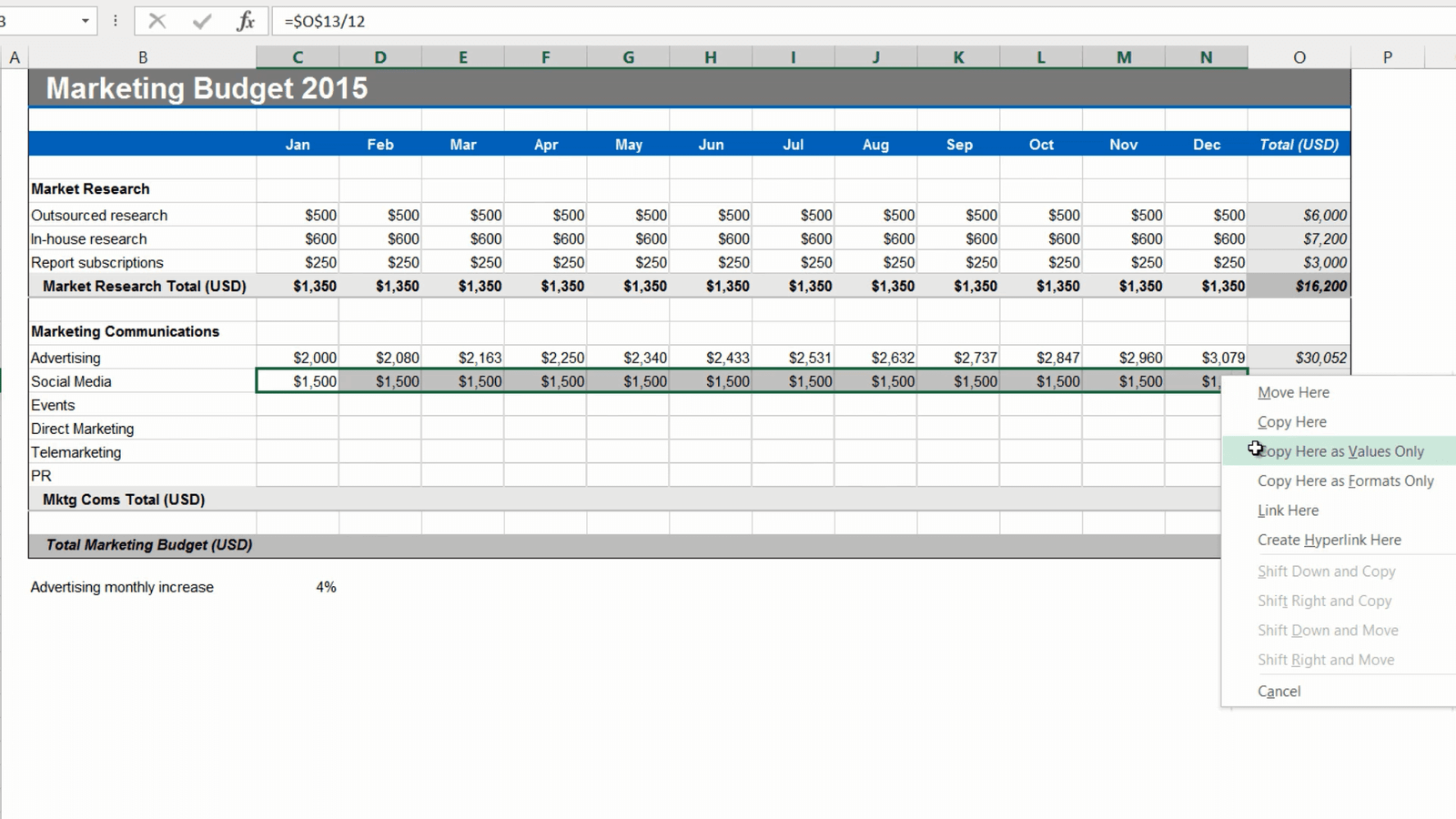
Next is “Social Media”. I want to spend 15,000-20,000 dollars on an annual basis distributed evenly throughout the year. I’ll start by entering 15,000 in the total cell and then in the cell for January I’ll write the formula, equal sign, mark the total and I want to make this absolute so I’ll click F4, and then divided by 12 for the 12 months.
If you hold down “CTRL” when you press “Enter” you’ll stay in the current cell. Now I’ll apply this formula to the rest of the months.
The monthly spend is 1250, I want to increase it a bit so I’ll change the year total to 18000. Now the monthly spend is 1500 which is better.
Now I need to remove the formula and only keep the values, otherwise if I later on manually change the value of a cell the total won’t update. To remove the formulas and only keep the values of these cells I’ll mark the numbers, right click, drag a little back and forth and then select to “Copy here as values only”.
If I double click you can see that the formula is gone, and only the values remain. I will go to the Total cell and remove the fixed value. Here I’ll use the keyboard shortcut for “AutoSum” which is “ALT + =”. And now, as you can see, if I make changes here in the cell the total is calculated correctly.
Selecting and filling random cells with a value (07:40)
On the next row I have “Events”. We plan to have our events quarterly. To fill multiple cells with the same value, hold down the “CTRL” key while marking the cells you want to fill. Here I’ll mark the cell for February and then mark a cell each quarter. Release “CTRL” and enter the amount you want to fill the cells with. Here I’ll write 1200. Press “CTRL” again and press “Enter”. All the cells that were marked are filled with the value.
Now I’ll continue to fill out the remaining line items.
Adding a “0” to empty cells (08:13)
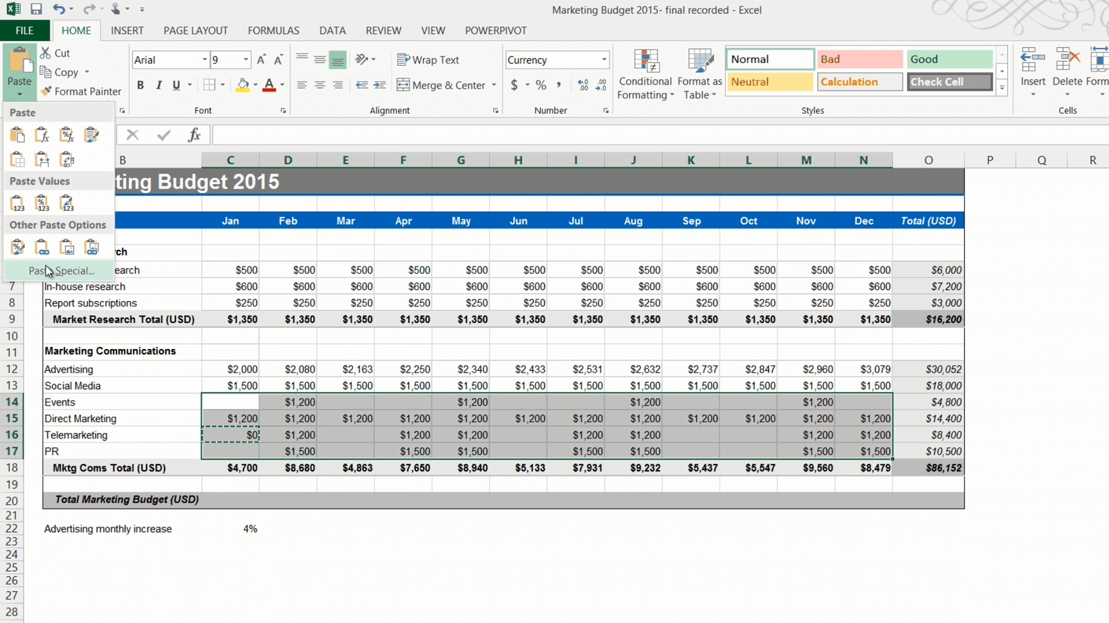
Now I’m almost done with my budget, I just want to add zeros to the remaining empty cells. Instead of manually filling out these cells, you can use a little work-around.
To fill multiple, random cells with zero, type 0 in one of the empty cells. Right-click and copy. Then mark the entire data range with empty cells that you want to fill, click paste and select “Paste Special”. Under “Operation” click “Add” and then “OK”. There, now zero has been added to all cells.
Now for the final row. Here I’ll enter a formula that add the first subtotal for “Market research” with the second subtotal for “Marketing Communications”. I’ll copy the formula across and select “Fill without formatting” since I only want to copy the formula. Finally I’ll hide the row with the advertising increase by right clicking and selecting “Hide”. There now I’m done with my budget!
Closing (09:11)
As you can see, by knowing how to use simple formulas and some of the shortcuts I showed you here, you’ll save a lot of time when filling out your spreadsheets.



Leave a Reply