
Easily navigate a spreadsheet
Introduction (00:04)
The first step for becoming really proficient using Excel is by knowing how to effectively navigate a spreadsheet. In this video you’ll learn how to quickly get a good overview of the contents of your spreadsheet, how to freeze rows and columns, how to navigate between different worksheets and how to compare them side by side. Let’s have a look!
Changing the way the menu appears (00:27)
Here I have our Marketing Budget for year 2015. When you first open up a spreadsheet it’s good to have a look around to get an overview of what the spreadsheet contains. To see more of the contents of your spreadsheet click the “Ribbon Display Options” button in the top right corner. To dedicate your full screen to the spreadsheet select “Auto-hide Ribbon”.
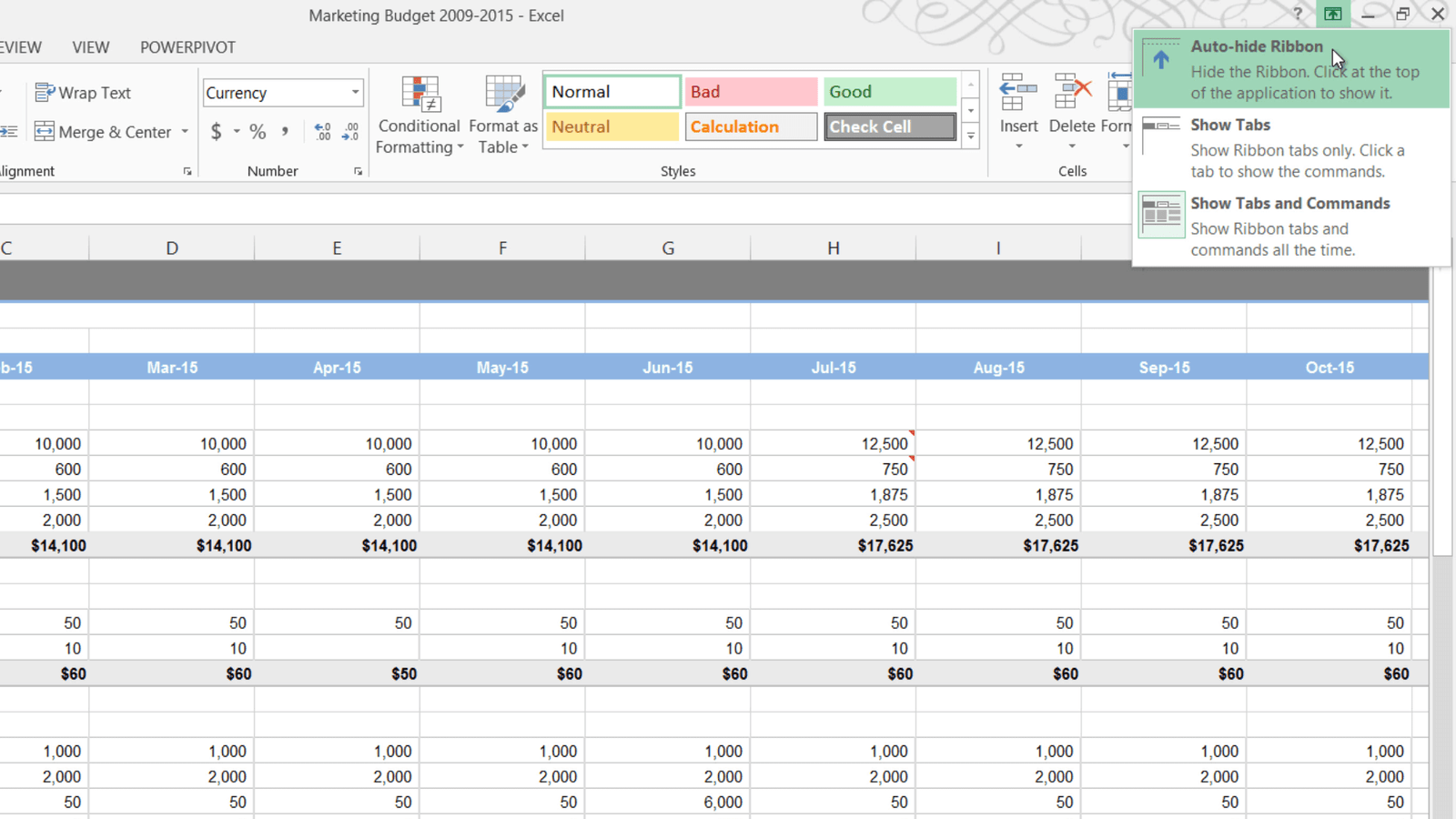
This replaces the Full Screen View that was available in previous versions of Excel. To open up the menu bar again just click the bar at the top, to make it disappear again click anywhere in your spreadsheet. The second option is to show only the tabs. To open up the commands just click on one of the tabs. The third and probably most used option is to always show the tabs and commands. You can easily switch between the two latter options by double-clicking one of the tabs, or by pressing the keyboard shortcut CTRL F1.
Navigating worksheets (01:30)
This spreadsheet contains multiple worksheets. You can easily select another worksheet by clicking on the desired tab. If you’re unable to see all tabs you can reduce the size of the scroll bar by holding down the left mouse button and dragging the three vertical dots to the right. Alternatively you can press the arrows in the bottom left corner to move the tabs left and right.

If you right-click one of the arrows you will see a list of all the worksheets and you can easily open one up by just double-clicking it in the list or selecting one and clicking “OK”. You can also use the keyboard shortcut CRTL Page Down to walk through each worksheet from left to right and press CTRL Page Up to walk through the worksheets from right to left.
Navigating columns and rows (02:21)
This spreadsheet isn’t very large so I can easily see how many rows there are by just scrolling down. If however, you have a very large spreadsheet it can be quite time consuming to scroll to the very end. To quickly get an overview of all the data in a spreadsheet press the keyboard shortcut CTRL End to go to the last row and column. To go back to the top again press CTRL Home. To go to the end of a cell range you can double click the corresponding border of a cell. If I want to see the total budget for salaries here I’ll just double-click the right border of the cell to go to the far right.
Similarly I’ll double-click the left cell border to go back to the far left. The same goes for going to the bottom or top of a cell range. You can also use the keyboard shortcuts CTRL arrow right, CTRL arrow left, CTRL arrow down and CTRL arrow up to accomplish the same thing.
Zooming in and out (03:20)
If you want to change the display size of the contents in your spreadsheet you can zoom in and out. To make the numbers in your spreadsheet appear larger, mark the cell that you want to see in the top right corner and then zoom in by dragging the zoom slider in the bottom right corner to the right.
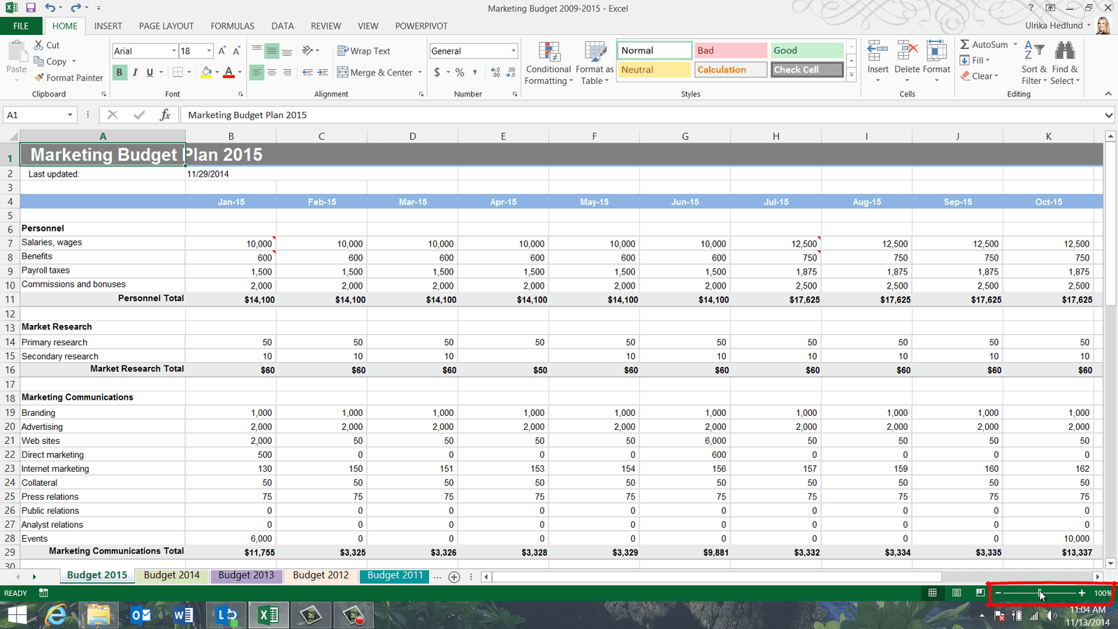
Another quicker way to zoom in and out is to hold down the CTRL key on your keyboard while turning the wheel on your mouse. If you have a touch pad you can zoom in by moving two fingers apart and zoom out by pinching them together.
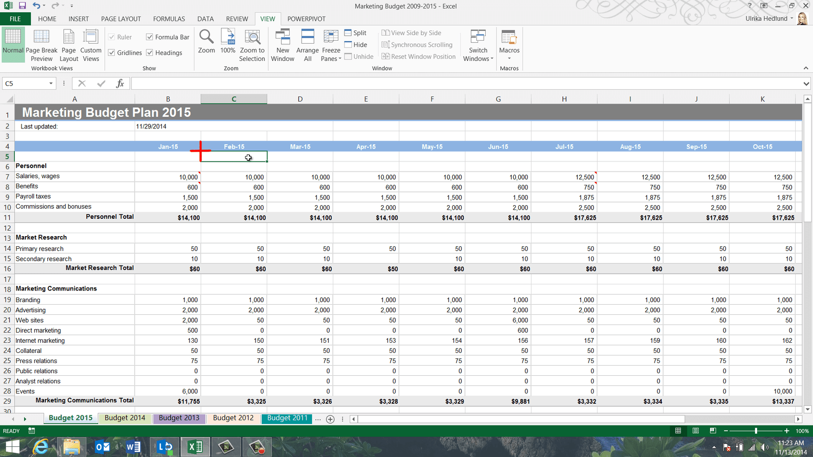
If you want to focus in on a specific area of your spreadsheet – here for example I want to look at personnel costs for the first quarter, mark the range of cells you want to focus in on, go to the “VIEW” tab and click “Zoom to Selection”.

Now I get a very focused view on those particular numbers. To zoom back out again I’ll just click the 100% button on the “VIEW” tab.
Freezing rows and columns (04:18)
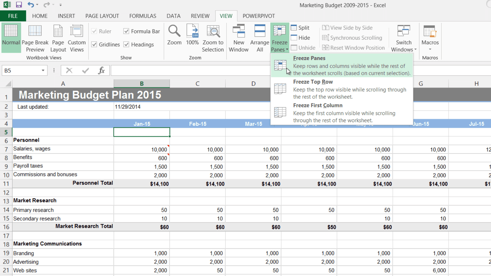
When I scroll to the right in the spreadsheet it’s hard to know which row a certain cell belongs to. To always see your row or column headings you can freeze panes. To freeze a row or column, on the “VIEW” tab, under the “Window” section click “Freeze panes”. Here I’ll select to Freeze the first column.

Now I can scroll to the right and still see the row headings. Now I want to do the same for the column headings. I have the option here to “Freeze top Row”, however in this case this doesn’t really help me because I have my column headings on the 4th row. I’ll go back and select to “Unfreeze Panes”. To freeze any row of choice, mark the row underneath the one you want to show, click “Freeze Panes” again and select “Freeze Panes”.
Now you can see that that the 4th row has been frozen and I can scroll down and still see which column belongs to which month. To freeze both the row that has the column names and the column that has the row names mark the cell to the right of the column and underneath the row you want to freeze and select “Freeze Panes”.
Now both the row and the column headers keep still when I scroll my document.
Hiding columns, rows and sheets (05:40)
Here I have a column where I’m just calculating the marketing budget increase from the year before. If I don’t want this to be visible in the report I can select to hide this column. To hide a column, right-click and select “Hide”.
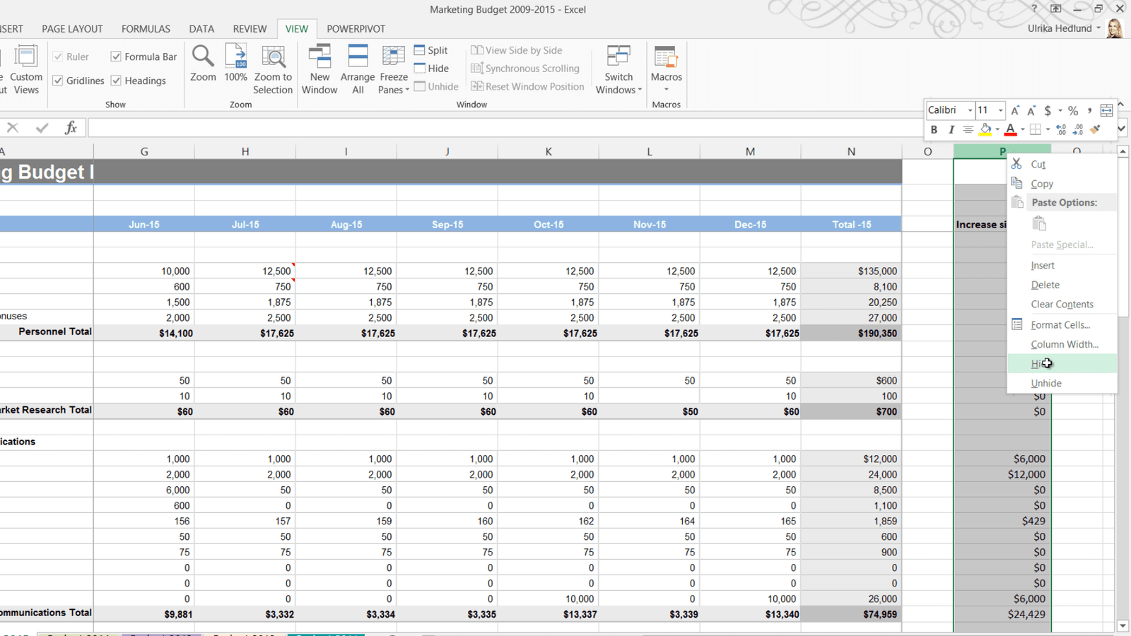
You can see that the column is hidden because there is a gap between O and Q. In Excel 2013 hidden columns and rows are easier to spot since they are also shown with a double line.

Now I only want to show the last quarter so I’ll mark the nine first months, right-click and “Hide”. To mark multiple, un-adjacent rows or columns hold down the CTRL key on your keyboard. Here I’ll mark all the budget item rows where we haven’t allocated any money in the budget. I’ll release the CTRL key, right-click and select “Hide”.
To get a better overview of all hidden rows and columns, on the “HOME” tab, click “Find & Select”, “Go To Special” and select “Visible cells only” and click “OK”.
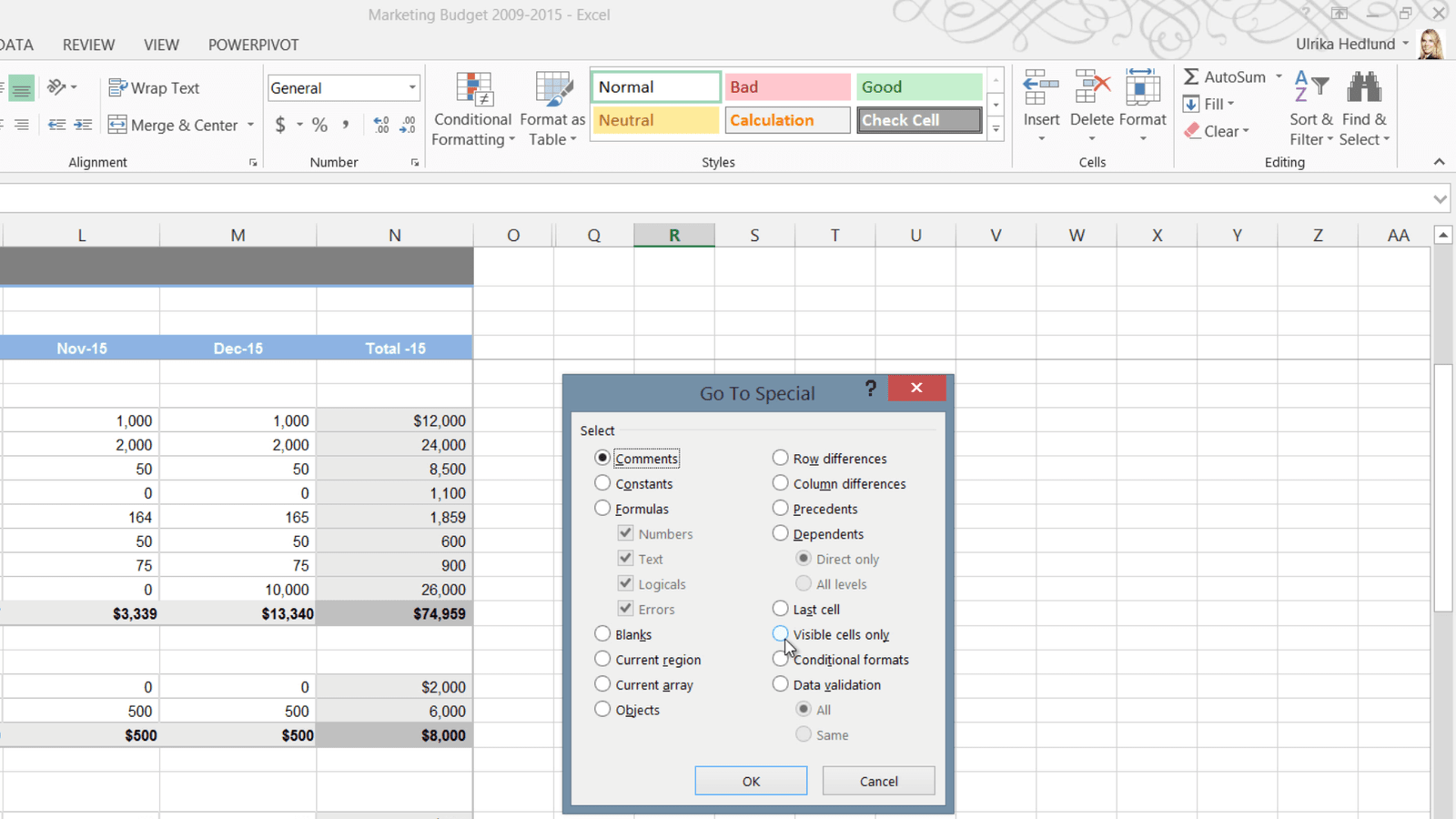
As you can see all hidden rows and columns are marked with white lines, making them easier to see.

To unhide a row, mark the adjacent rows, right-click and select “Unhide”, or just double-click the hidden row. The same goes for un-hiding columns.
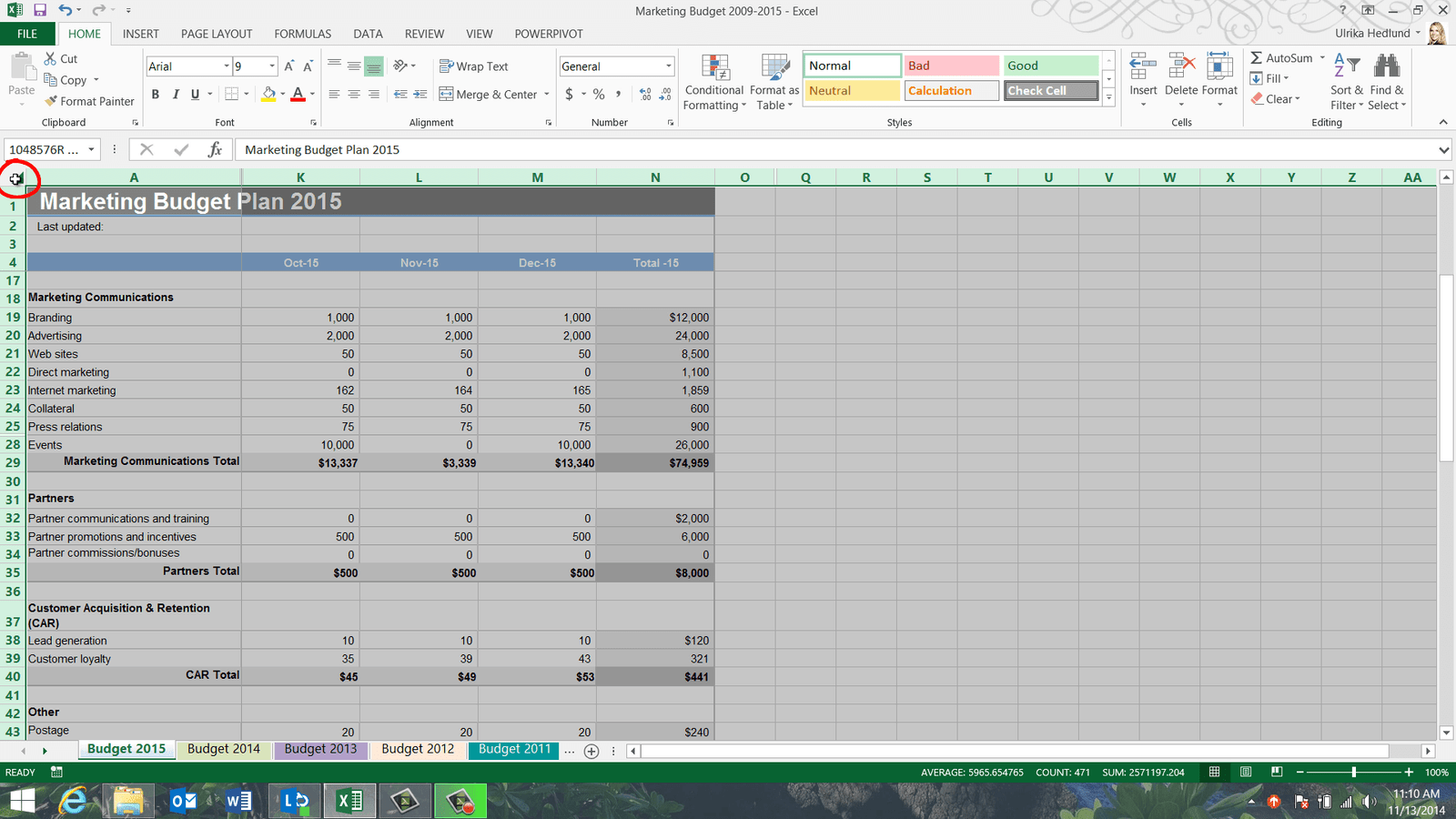
If you want to unhide all hidden rows and columns at once, mark the entire worksheet by clicking the top left corner between A and 1.
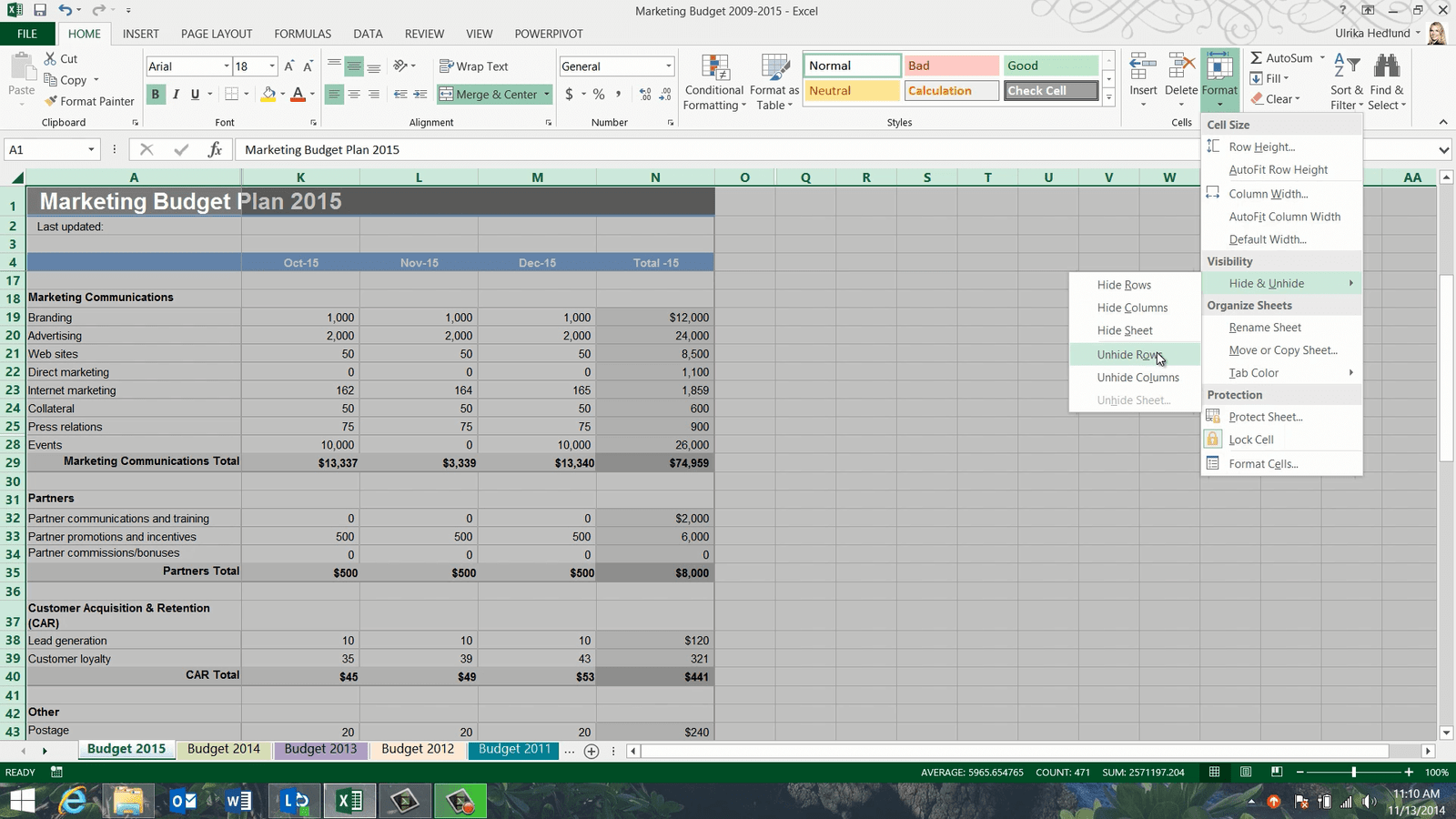
On the “HOME” tab, in the “Cells” section, click “Format”, “Hide & Unhide”, and then select “Unhide Rows” and then select “Unhide Columns”.
You can also hide entire worksheets. To hide the budget for 2009, I’ll step to the right to make the worksheet visible. I’ll right-click the sheet tab and select “Hide”. To unhide it, I can click any sheet and click “Unhide” and select the hidden worksheet that I want to show again.
Using split panes to compare rows and columns (07:47)
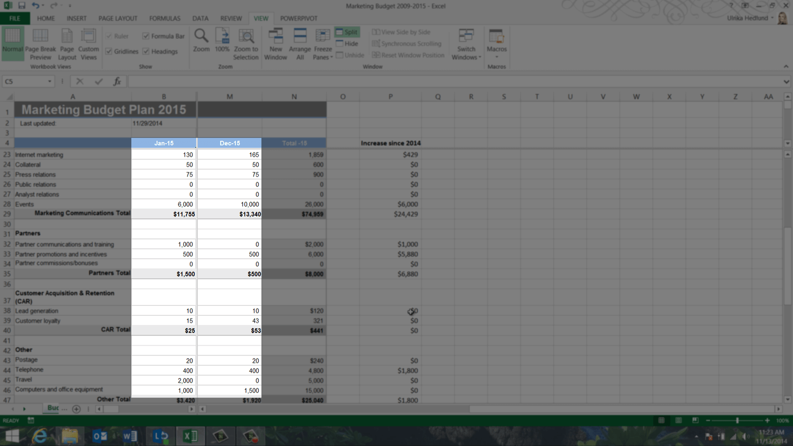
Now I’d like to compare the budget for the month of January with the month of December. To easier compare columns side by side I’m going to split my window into multiple panes. To split your spreadsheet into multiple windows, mark the cell underneath to the right of where you want to place the center of the split, on the “VIEW” tab click “Split”.
At the bottom of the spreadsheet I have two independent scroll bars. I’ll scroll to the right in the right pane so that I can see the month of December. Now it’s much easier for me to compare January and December side by side.
If I want to compare any other months side my side I can easily move the split and scroll each pane. To remove the splits on the “VIEW” tab click “Split” again, or just mark the center of the split and double-click.
View worksheets side by side (08:41)
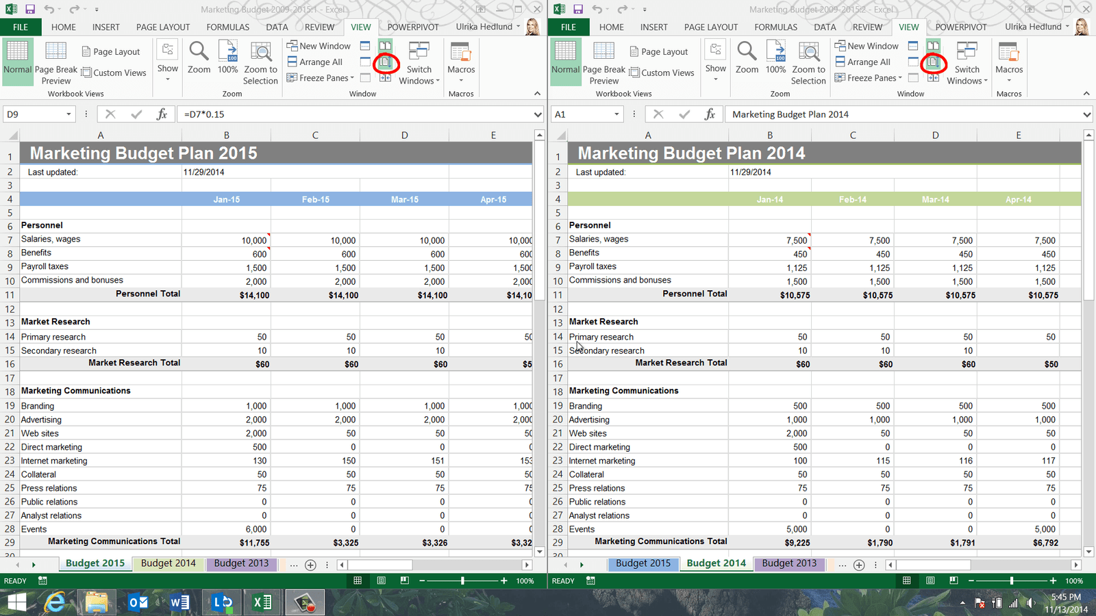
Now I want to compare the budget for 2015 with the budget for 2014. To compare two worksheets side by side, on the “VIEW” tab click “New Window”.
Excel opens up a second window showing the same spreadsheet. Unlike in previous versions, each window in Excel 2013 has its own menu bars so that it’s easier to work on multiple monitors. In the window marked with colon 1 I’ll open up the worksheet with the budget for 2014. To see these windows side by side on the “VIEW” tab click “View Side-by-Side” and make sure that “Synchronous Scrolling” is turned on under the “VIEW” tab to scroll both windows simultaneously.
Now I can easily compare the windows side by side. If I want to scroll each window independently I’ll click “Synchronous Scrolling” on the “VIEW” tab to turn it off, and then I can scroll them one by one. To go back to the original view, just close down one of the windows.
Closing (09:50)
By knowing how to effectively navigate a spreadsheet you’ll be much more proficient using Excel.
Leave a Reply