Rearrange and clean up your data
Introduction (00:04)
From time to time you need to re-arrange data and clean it up in your spreadsheet in order to display it the way that you want it. In this video you will learn how to re-arrange rows and columns, how to spot and remove duplicates and how to change data types for easier analysis. Let me show you!
Changing column and row width (00:24)
Here I have a spreadsheet with customer prospects that we are going to share with an agency for follow up. I’ve been given another spreadsheet with additional prospects that I need to add to my list. But the data in this additional spreadsheet is arranged differently and there might be duplicates so I need to clean up the data before I can consolidate the lists.
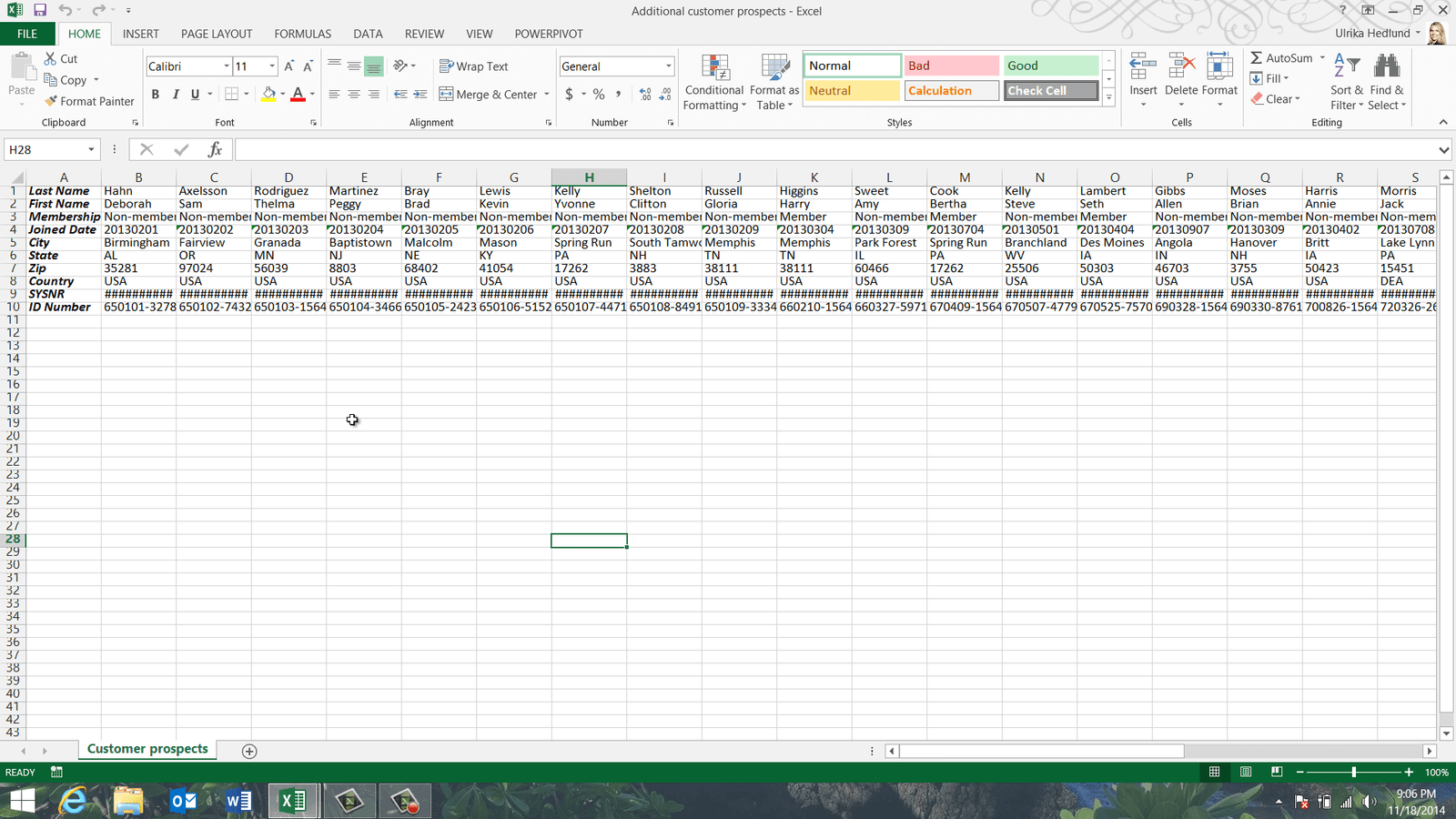
The data in the second spreadsheet is very compressed. Here is a row that only seems to contain hash tag symbols.
This is Excel’s way of telling you that the cell is too small to display the full contents. You can make the column wider by dragging the column edge to the right to see the full contents.
Instead of resizing individual columns you can resize all columns and rows at the same time. To change the width of all columns, mark the entire spreadsheet and then make any column wider, all columns will then have the same width. You can also double click between two columns to automatically make the columns as wide as they need to be to properly show the contents. You can do the same for the rows by double-clicking between two rows. As you can see the entire spreadsheet is now much easier to read.
Turning data from row to column (transposing data) (01:44)
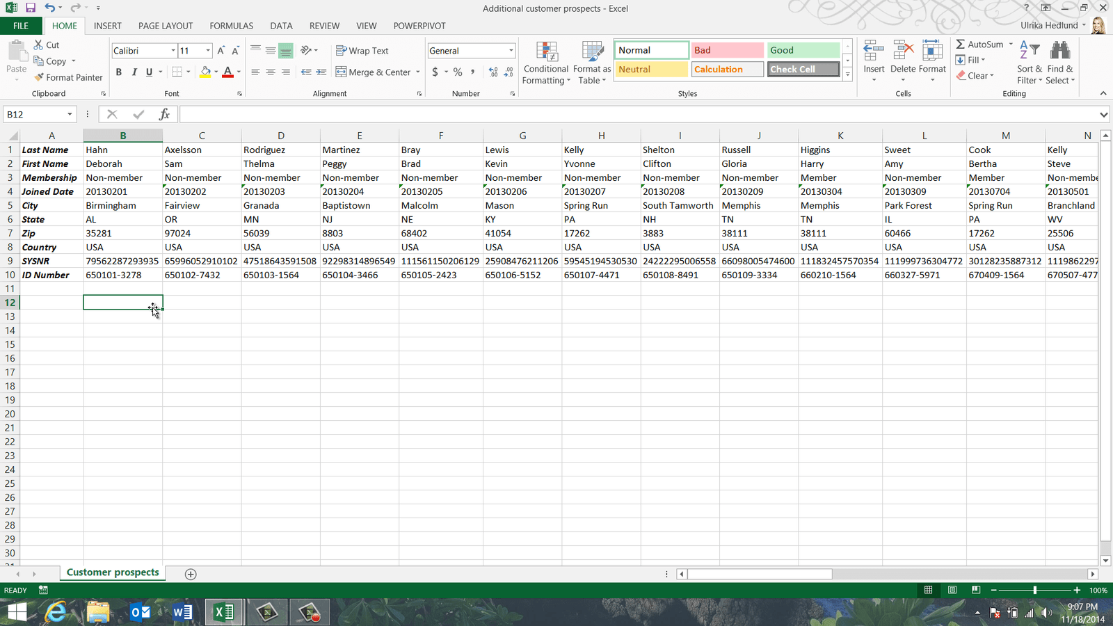
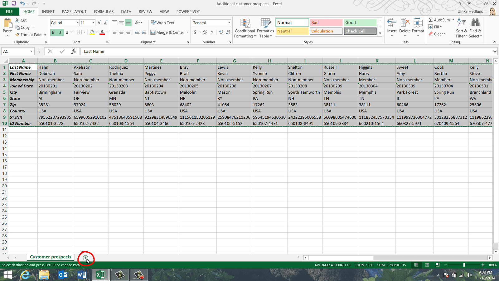
Now I can see that the layout of this data is different than in my original list. To append this list to mine I first need to convert the rows into columns –that is transpose the data. To transpose data, first mark the entire data range by marking the first cell and then pressing the keyboard shortcut CTRL Shift End. Right-click and select “Copy”. I’ll open up a new worksheet by clicking the plus sign at the bottom of the spreadsheet.
To re-arrange the data from row to column layout, right-click and under “Paste Options” select “Transpose”. The data is copied and turned from column to row.
Comparing spreadsheets side by side (02:30)
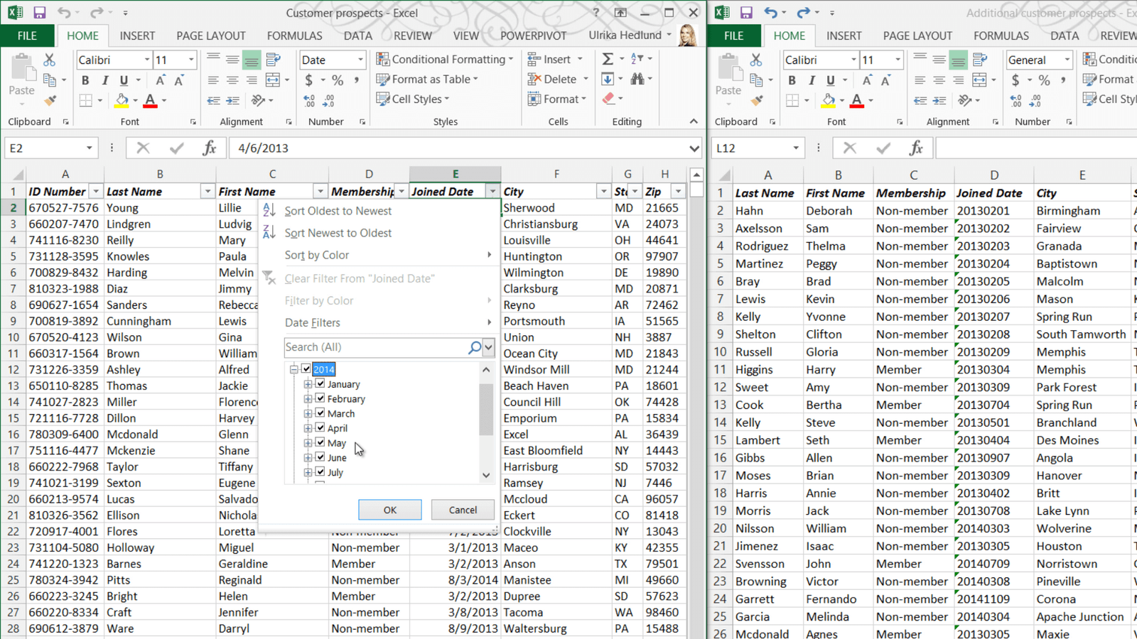
Again, to change the width of the columns I mark the spreadsheets and double click. Before I copy data to the other spreadsheet I need to make sure that the spreadsheets contain the same columns and that they are in the same order. To compare the spreadsheets side by side I’ll press the keyboard shortcut Windows key Arrow Right to move this windows to the right, then I’ll mark my other spreadsheet. Instead of using the keyboard shortcut I can use the mouse and drag the window to the left side of the screen. Here I can see that my initial list doesn’t contain the column named “System Number”, my original list also has the ID number as the very first column.
In my original spreadsheet the contents of the “Joined Date” column is stored as dates. This means that I can easily filter the list by “Joined Date”.
In the second spreadsheet the data is stored as “Text”. If I go to the “DATA” tab and select “Filter” and look at the “Joined Date” column you can see that I just get a long list of numbers, Excel doesn’t treat the data here as dates.
I’ll cancel here and remove the filter from my list. To make the necessary fixes to this spreadsheet I’ll maximize the window again by clicking “Maximize” in the top right corner.
Deleting and moving columns (03:58)
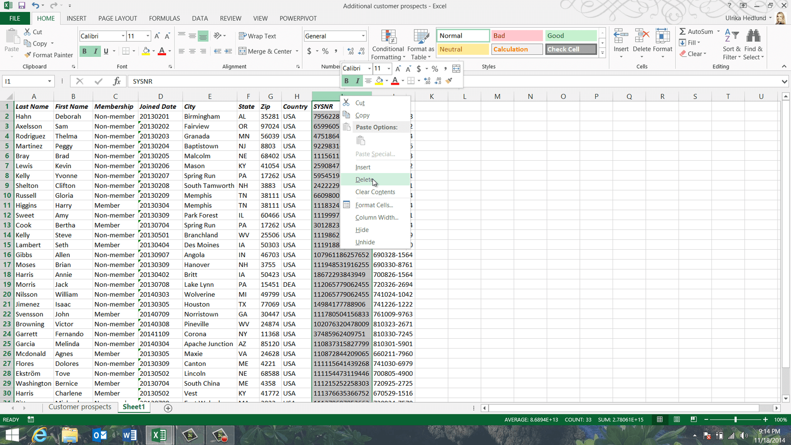
To delete a column, right-click the column heading letter and select “Delete”.
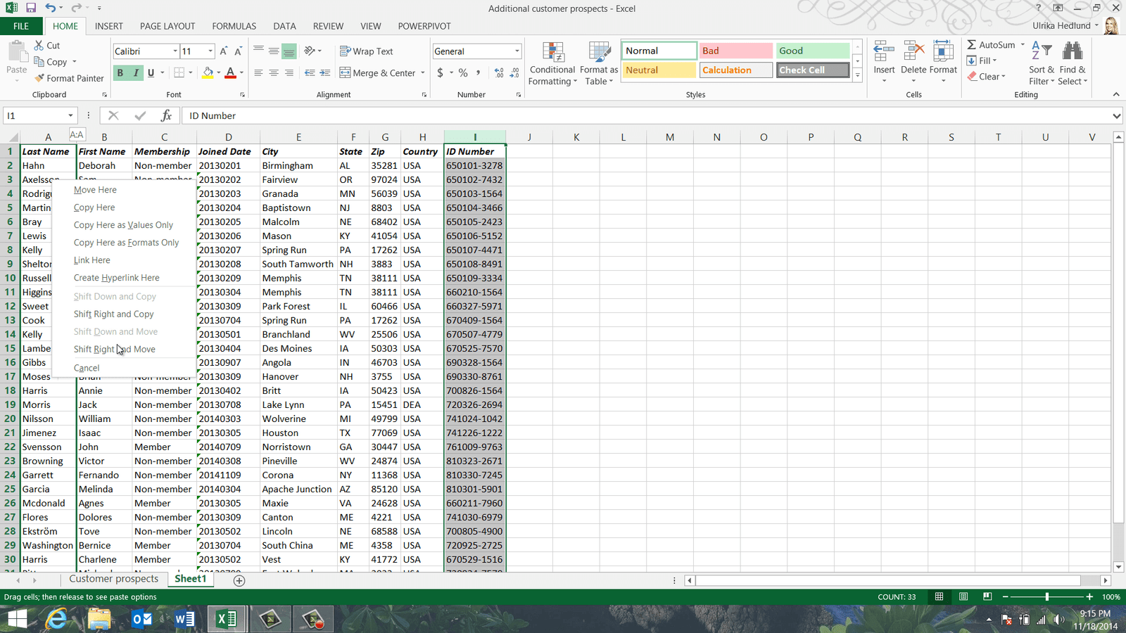
To move a column, mark the column by left-clicking the column letter, move your mouse cursor to either side of the column until you see a cross, hold down the right mouse button and drag the column to the desired position, release the mouse button and from the menu select “Shift Right and Move”.
The columns are shifted to the right to make room for the ID Number column.
Changing column data type (04:32)
To convert the data type of the “Joined Date” column from Text to Date mark all cells that contain the text string by marking the first cell and then pressing CTRL SHIFT Arrow Down on your keyboard. Click the “DATA” tab and then in the “Data Tools” section click “Text to Columns”. A wizard opens up that steps you through the process. In the first step you are asked about delimiters. You don’t have to change anything here so click “Next” to go to the next step.
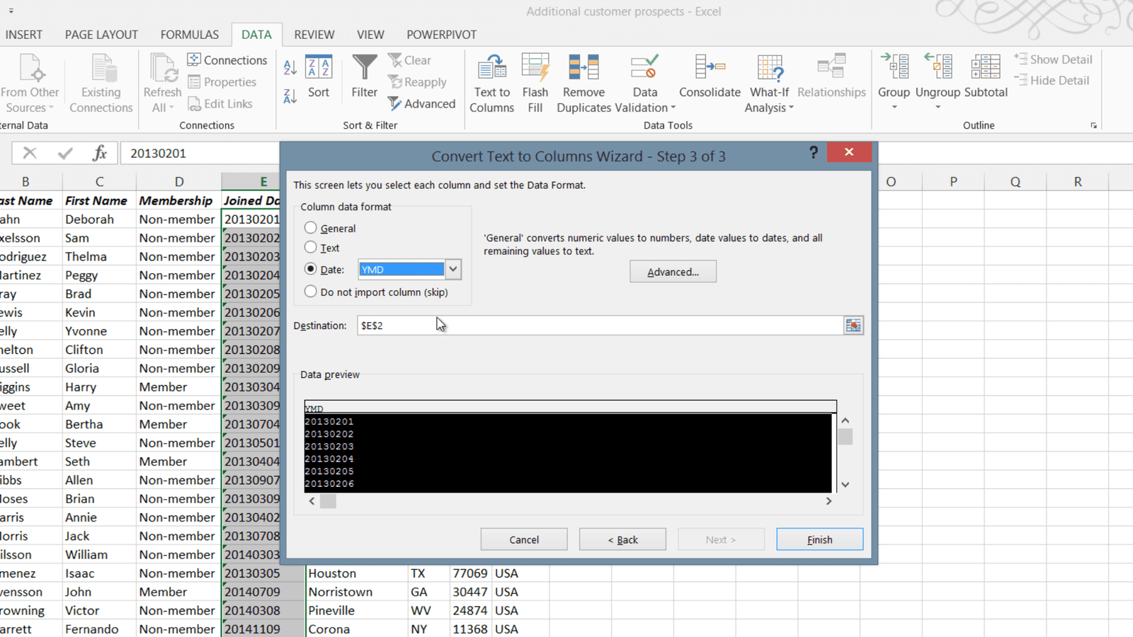
In the second step uncheck all delimiters, since the text string is all in a single string. In the third step of the wizard you have the option to set the data format. Select “Date” and specify the format as Year, Month and Day (YMD) since this is the way the text string is written and then click “Finish”.
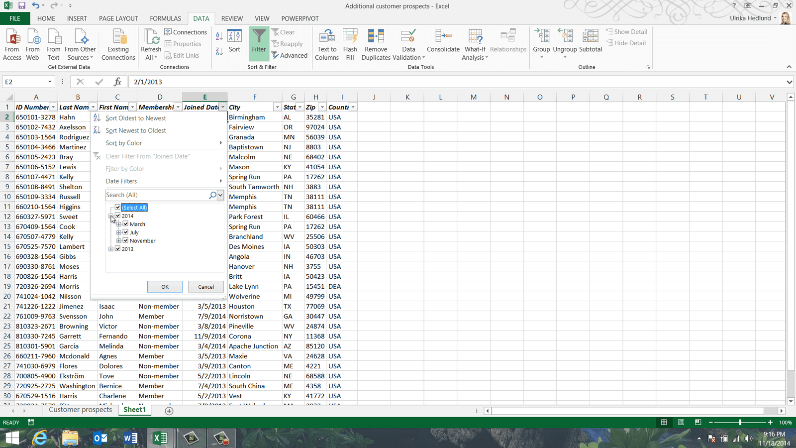
As you can see the format of the “Joined Date” column has now been changed and if I click on the “Filter” button I can select to filter this column on a specific year or month.
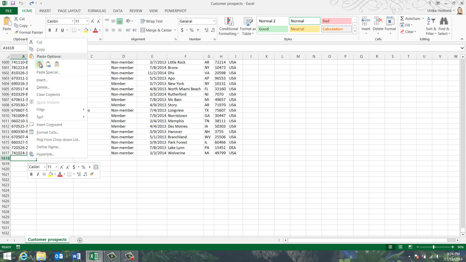
Now I can copy the data over to my original spreadsheet. Before I do, lets save the changes to my spreadsheet. To copy the full data range I’ll mark the first cell under the heading row and press CTRL Shift End on my keyboard. I’ll right-click and select “Copy”, next I’ll open up my original spreadsheet and go to the very end by pressing CTRL End. I’ll mark the first empty cell under my list, right-click and select “Paste”.
To go back to the top again I’ll press CTRL Home. Now I have all data consolidated in one spreadsheet. Now I just have to make sure I don’t have any duplicates.
Spotting and highlighting duplicates (06:23)
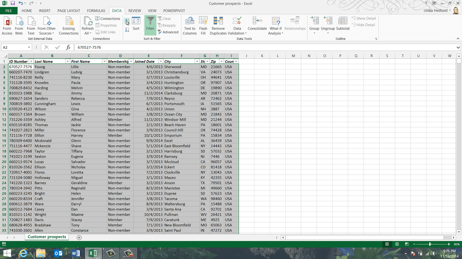
To easier spot duplicates start by sorting your data on unique values. In this list two people might have the same first and last name, but the “ID Number” for everyone is unique. To sort on the “ID Number” column I’ll mark a cell in this column, click the “DATA” tab and then sort A to Z.
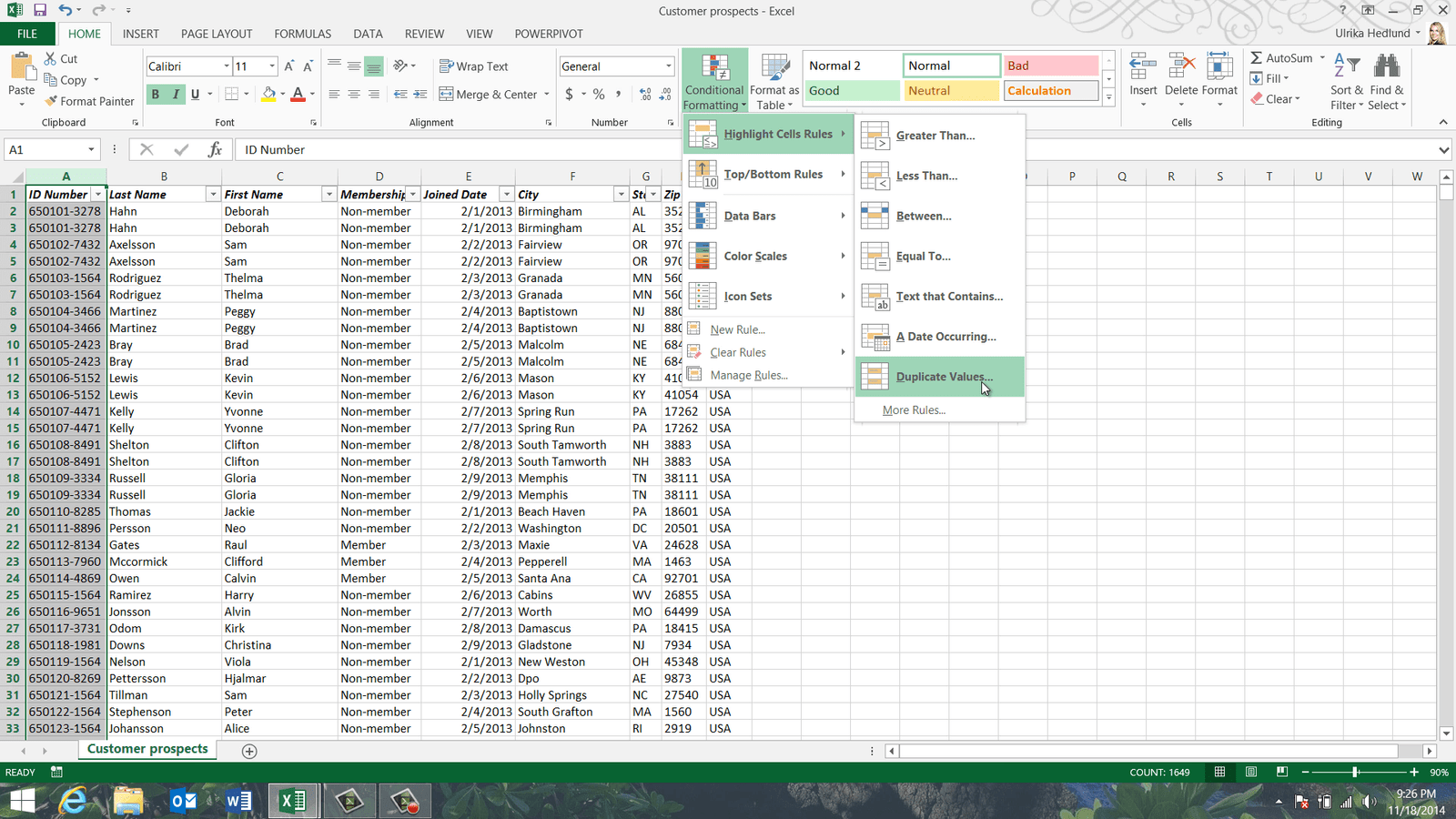
I can immediately see from just looking at the data that I do have duplicates. To make duplicates stand out even more you can highlight them using conditional formatting. Mark the column where you want to highlight duplicates, in my case it is the first column with the “ID Number”. On the “HOME” tab, click “Conditional formatting” and select “Highlight Cells Rules”, and then “Duplicate Values”.
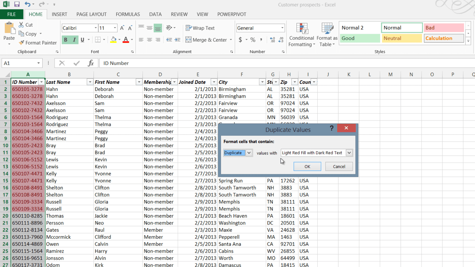
Here you can select how you want the duplicates to be formatted, I’ll just leave the default coloring which is light red fill with a dark red text.
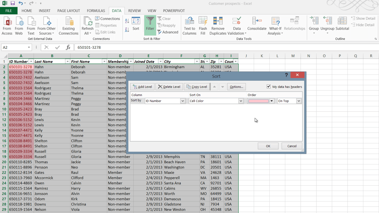
I’ll click “OK” and now the duplicates in my dataset are clearly visible. If I scroll down I can see that I have even more duplicates further down in the list. To see all duplicates at the top you can sort by color. Click the “DATA” tab, and in the “Sort & Filter” section click the “Sort” button. Instead of sorting the “ID Number” column by “Values, I’ll change the “Sort On” drop down to “Cell Color”, in the “Order” drop down I’ll select the red color and then leave the default which is “On Top”.
Now all duplicate records are sorted on the top. I’ll mark all colored cells and can see in the bottom of my spreadsheet that the cell count is 46, which means I have 23 duplicate records.
Automatically removing duplicates (08:12)
Instead of manually marking and deleting the duplicates I can use a built in tool in Excel. To automatically remove duplicates, mark any cell in your dataset, on the “DATA” tab in the “Data Tools” section click “Remove Duplicates”. Here I’ll leave the check box that says “My data has headers” marked. Leave all the columns checked to only remove rows where the values in all columns are the same, and then click “OK”.
As you can see, Excel removed 23 duplicate records. Now I’ll save this as a new consolidated list. I’ll click “FILE”, “Save As” and then save my spreadsheet.
Closing (08:53)
By knowing how to re-arrange and clean up your data you will save a lot of time when working on large data sets.





Leave a Reply