
Modify data with Flash Fill
Introduction (00:04)
Quite often you have a spreadsheet with data that you need to modify in some way. In this release of Excel Microsoft has introduced a great new tool called Flash Fill to help you modify data. If you show Flash Fill what you want to change Excel understands the pattern and updates the data for you. In this video you will learn how to use Flash fill as well as traditional tools and formulas to modify your data.
Using Flash Fill to modify data (00:28)
Here I have a spreadsheet with customer leads that I want to modify a bit. First I want to change the “Name” column so that the letters aren’t all upper case. Instead I want it to look like this, with only the initial letter of the first and last name to be capitalized.
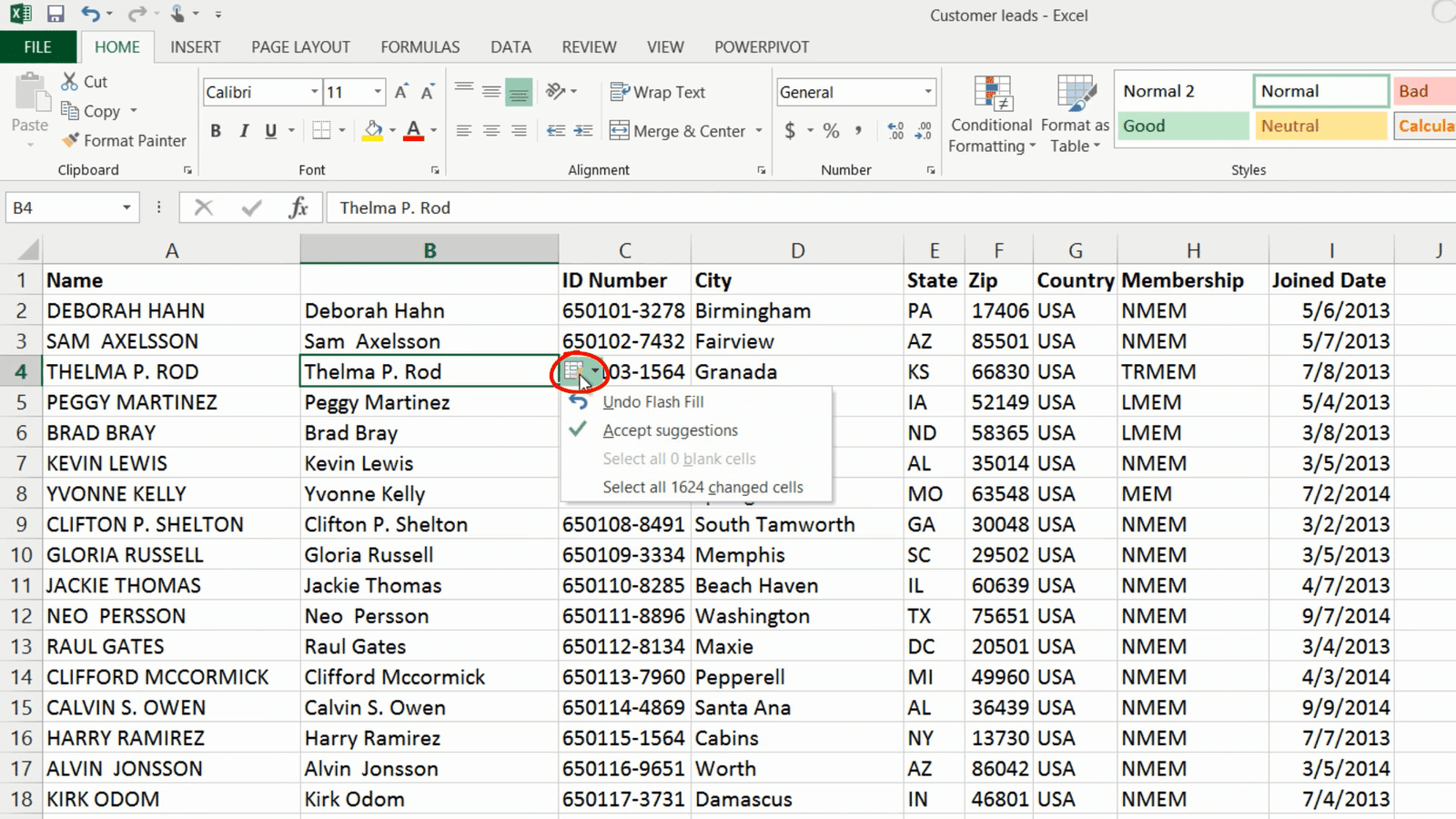
To use Flash Fill to modify the names in the first column so that they are not all in upper case, insert a temporary column by right-clicking and selecting “Insert”. Start typing the data the way you want it to appear. In this case, I only want the first letter of the first and last name to be uppercase and then the remaining lowercase. I’ll press Enter and continue with the next cell. Flash Fill automatically kicks in when Excel thinks it has understood the pattern, it suggests what the remaining cells should contain and to accept the changes just press Enter on your keyboard.
A little Flash Fill icon appears allowing you to accept or reject the changes. In this case I’m happy with the changes so I’ll click “Accept Suggestions. “
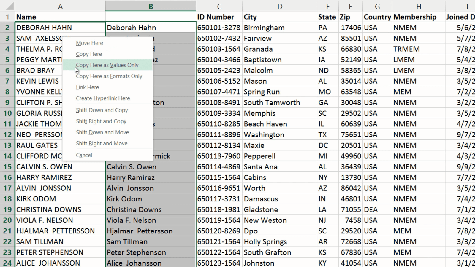
To copy the modified content to my original column, I’ll select the data range by marking the first cell and then pressing CTRL Shift Arrow down on my keyboard. I’ll hold down the right mouse button and move the contents to the first column, release the mouse button and select “Copy here”. I’ll press CTRL Home on my keyboard to go back to the top. Then I’ll just delete the temporary column by right-clicking the column header and selecting Delete.
Modifying data with simple functions (02:06)
Using Flash Fill you save a lot of time since you don’t have to figure out difficult formulas. In this case the function to use is quite easy if you know it. To convert text to proper case, write equal mark and then PROPER left parenthesis, mark the contents in column A and then press Enter. To copy the formula to all cells just double-click the bottom right corner. To copy over only the contents, right-click and move the data, release the mouse button and select “Copy here as values only”. That way the names, not the formula is copied over.
In this case using the function was very straight-forward, but in many cases even simple modifications require complex formulas. Let’s go back to the original spreadsheet to have a look.
Using Flash Fill to replace complex functions (02:55)
Say that in addition to changing the letters to proper case you want to remove any middle initials. Start typing the names the way you want them. Flash Fill suggests a modification but it hasn’t understood that you want to remove the middle initial. If you don’t agree with the suggested change just keep typing in cells the way you want them to appear.

Here I’ll write in the name without the middle initial and Flash Fill makes a new suggestion. This one is correct so press Enter to accept the change. If you wanted to make the same change without Flash Fill, you would have to use a very advanced formula. For example one that looks like this:
=LEFT(A2,FIND(” “,A2))&TRIM(RIGHT(SUBSTITUTE(A2,” “,REPT(” “,99)),99))
As you can see it’s quite complex and it takes some time to figure it out, so if you want to make modifications like this, Flash Fill is a great time saver.
Splitting a column into two using Flash Fill (03:44)
Now I want to split the Name column into two columns, one with the first name and one with the last name. I’ll insert two empty rows, I’ll mark the column to the right, right-click and select insert. To repeat the same step again press the keyboard shortcut CTRL Y. I’ll type in the headings for the columns, “First Name” and then “Last Name”. To use Flash Fill I will start typing in the first name. To automatically trigger Flash Fill without filling in additional columns, press the keyboard shortcut CTRL E.
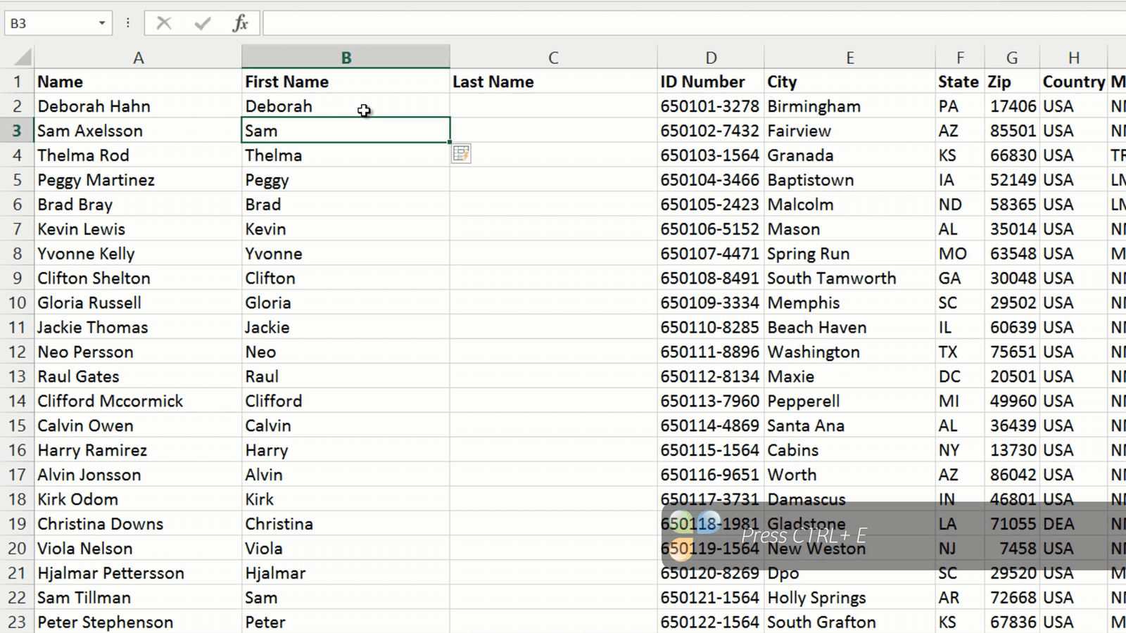
Flash Fill understand the pattern and fills in the first names for me. You can use Flash Fill even for columns that are not next to each other. In the Last name column I’ll write the last name from column A, then I’ll press CTRL + E on my keyboard to trigger Flash Fill. The last names are added to my Last Name column.
Splitting a column into two using “Text to Columns” (04:42)
If you want to split the contents of one column into multiple columns without using Flash Fill you can use the Text to Columns wizard. To split a column into multiple columns, mark the contents of the column you want to split, in this case I’ll mark the contents of the “Full Name” column by marking the first cell that contains the name and then pressing CTRL Shift Arrow Down. Go to the “DATA” tab and click “Text to columns”.
In the first step, just leave the default which is “Delimited”, and click “Next”. In the second step you need to tell Excel how the data should be separated; in this case the first and last name are separated with a space so I’ll deselect the tab separator and instead select the checkbox for “Space”. You get a preview of what the data will look like to make sure that it looks the way you intend.

Click “Next” to go to the final step. Here you need to enter the destination for the split columns. Mark the first cell in the column where you want the split data to appear and then click “Finish”. Now you can see that your data has been split into two columns.
Combining data from multiple columns into one (05:54)
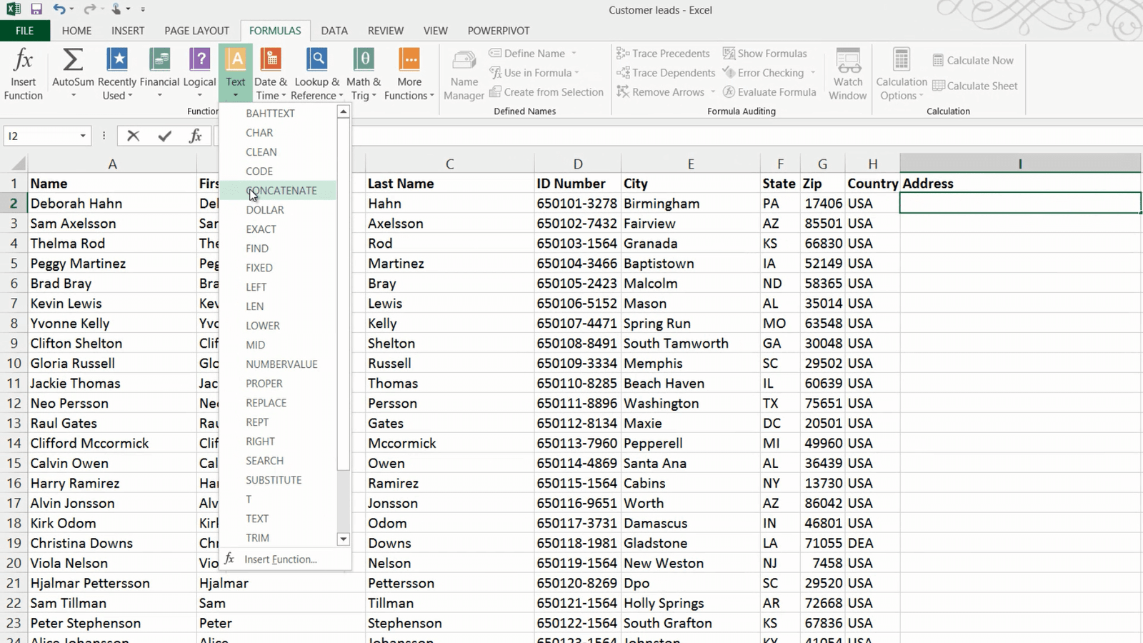
Now I want to add a column called Address that combines the data from the four columns “City”, “State” “Zip” and “Country” into one single cell. If a value is changed in any of these four columns I want the Address column to update automatically which means I can’t use Flash Fill, since Flash Fill only works on existing data, not future changes, so instead I will use a formula to achieve this.
To combine contents from multiple columns into one, mark the cell where you want your results, on the “FORMULAS” tab, click the Text library and select “CONCATENATE”.
Finding functions (06:34)
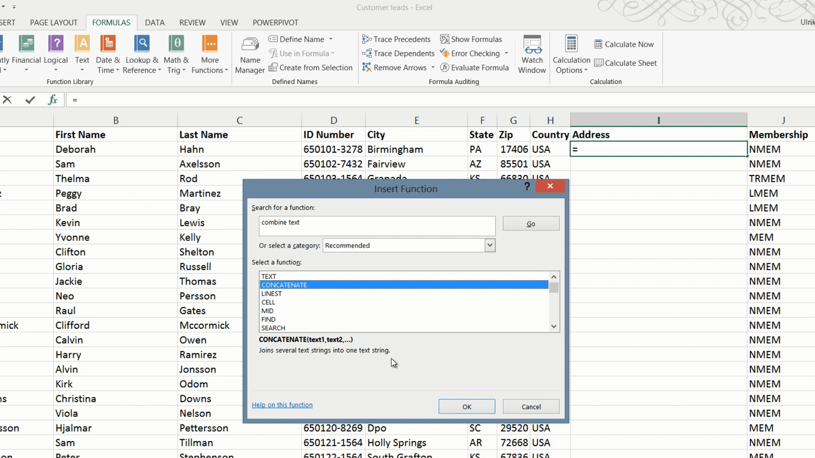
If you don’t know what function to use you can search for it and Excel will give you suggestions. To search for a function, on the “FORMULAS” tab click Insert function. Write a short description of what you want to do, here I’ll write “combine text” and then click go. Excel provides you with a list of options and you can see a short description of what the function does. The first one is not right, but the second Concatenate joins text strings together which is exactly what I want to do, so I’ll click OK.
In the formula windows you get to enter the text strings you want to combine. Here I’ll start with “Text1” which is the city name so I’ll mark cell E2, then I’ll add a comma and space, the state name, another space, the “Text5” field should contain the ZIP code which is in G2, to add another text field press Tab on your keyboard. In the “Text6” field I will add a comma and space, press Tab again and mark the country field which is H2 and then I will click “OK.”

The address field is populated with the combined contents and I can copy the formula by just double-clicking the bottom right corner.
Another way to combine text strings is by using the “and” symbol (&) which does the same thing as the Concatenate function. Using the “and” symbol you the formula would look like this instead.
=E2&”, “&F2&” “&G2&”, “&H2
Now if new values are entered in any of the four columns the Address column will be automatically updated.
Replacing data in cells (08:13)
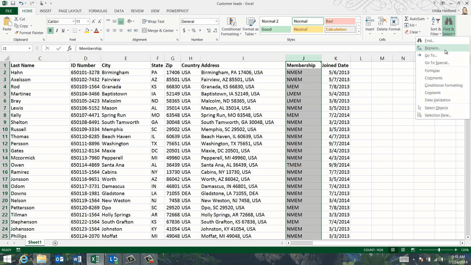
In the column named “Membership” I have a lot of abbreviations. I want to modify the contents of the column so that it looks like this instead. I could use Flash Fill but in this case it wouldn’t be very effective since I would have to write so many names manually to show the pattern. Here it is better to use Find and Replace. To use the replace tool, mark the data range where you want to make the replacements. Here I’ll mark the “Membership” column. On the “HOME” tab, in the Editing section click “Find & Select” and then “Replace”.
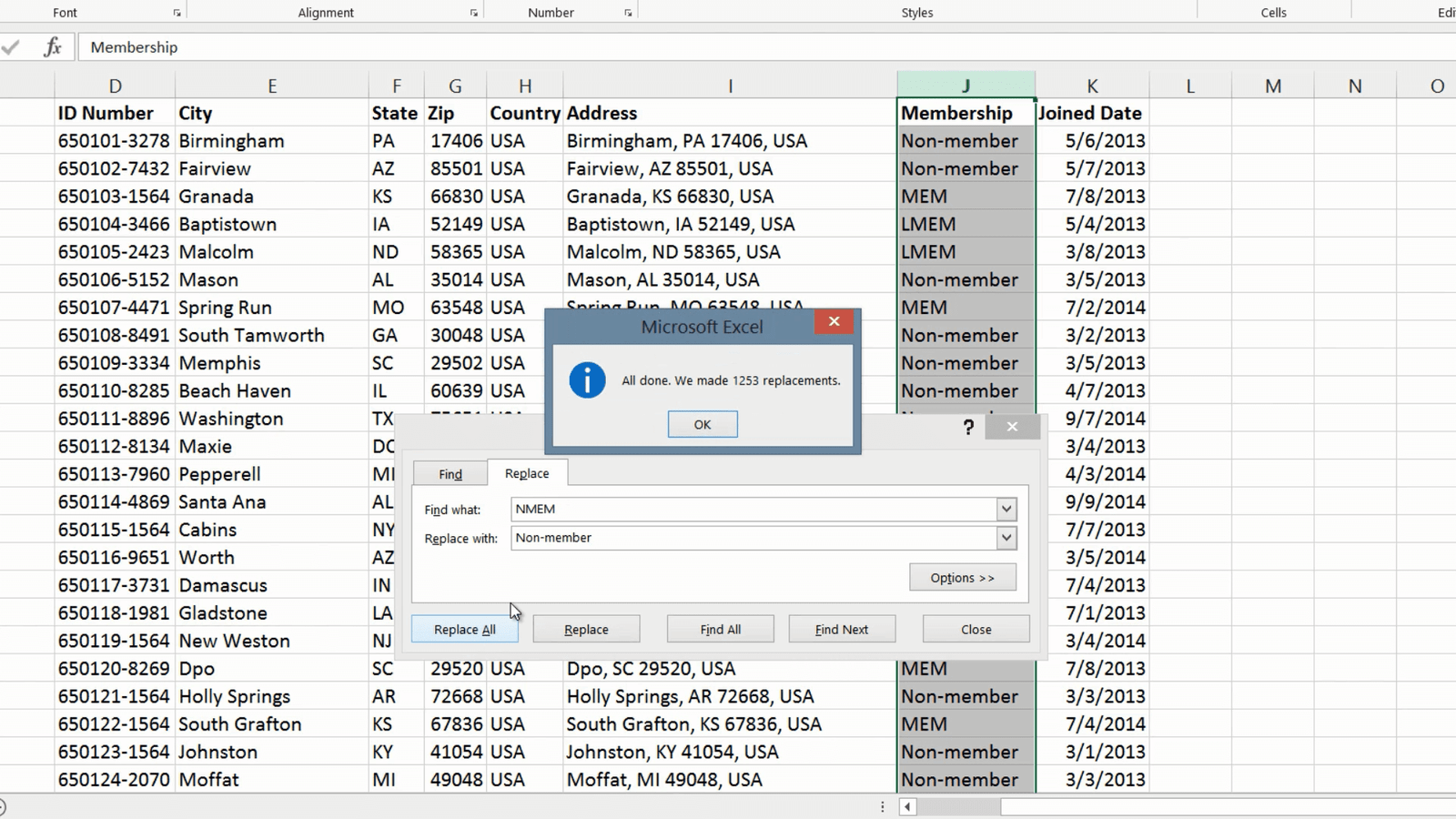
In the “Find what” text box type what you want to find, here I’ll write the abbreviation “NMEM” and in the “Replace with” text box type in what you want to replace it with, I’ll type “Non-Member” and then click “Replace All”. 1253 replacements where done I’ll click OK and continue with the next one.
Now I want to replace the abbreviation MEM with Member, but since this letter combination appears in other abbreviations as well I need to click “Options” and mark the option to “Match entire cell contents” then click “Replace All”. I’ll continue to make the replacements using the Replace tool until all the abbreviations are gone. Great, now the data is much easier to comprehend.
Closing (09:37)
By knowing how to use Flash Fill and other tools within Excel, you will save a lot of time when modifying your data.
Leave a Reply